Sequential Impulses explained from the perspective of a game physics beginner
INTRODUCTION AND PREREQUISITES
This article is meant to be a crash course to help you understand Sequential Impulses, a method of resolving collisions in a real-time physics engine. The idea is that by the end of it, you will hopefully understand this method in a way that will make you think: “I could have discovered this myself!”.
That being said, there are some prerequisites that I will be glossing over in this article,
- Linear algebra
- Kinematics
- Impulses and Momentum
- Some familiarity with derivatives
But with that out of the way let’s begin with actually defining the problem. Generally speaking, a physics engine would have 2 phases: Collision Detection and Collision Resolution. In this article, we will be treating collision detection as a black box. We have a set of bodies, they move and collide with each other, and our collision detection system is able to detect that.

But the problem is after finding the collision, and information regarding the collision such as the collision normal, the contact points, and all that, how would do we actually resolve the collision? Well, the first idea we need to understand is the idea of expressing the collision as a constraint.
EXPRESSING THE COLLISION AS A CONSTRAINT
What if we could describe how “deep” a collision is using a function?

What if we had some sort of function which we will call C and it takes in a set of parameters and it will output a single number. If the number is positive, there is no collision, and if there is a collision this number is negative. And the idea is that we also know how deep the collision is, it makes sense that the smaller the number the deeper the collision.
In order to find this mystery function, perhaps we could first look at a real example.

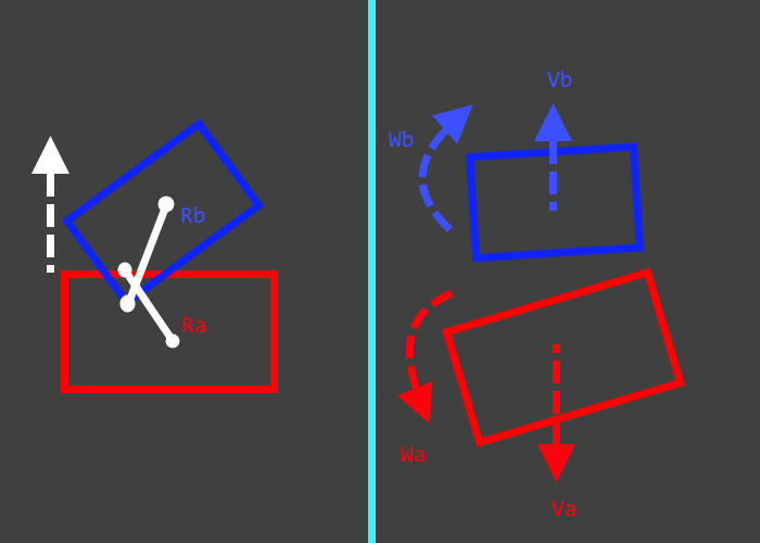
Imagine a collision between this block A and the rotated block B.

In this case, just by eyeballing it, we can clearly see that if we want to resolve the collision it makes sense that we would resolve this in the world up direction. In other words, this is the Collision Normal. Of course, we could use any direction, but we can see that it moves the least when we use the collision normal, it’s also a lot more physically based.
The contact points of the collision would be the parts of the body that penetrate the most.
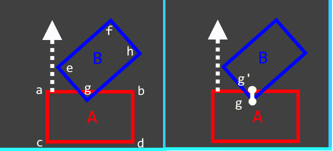
The contact points of the collision from the perspective of block B and would be point g. And the contact point of the collision would be g projected on the collision normal.
Using this information we can find this mystery function.
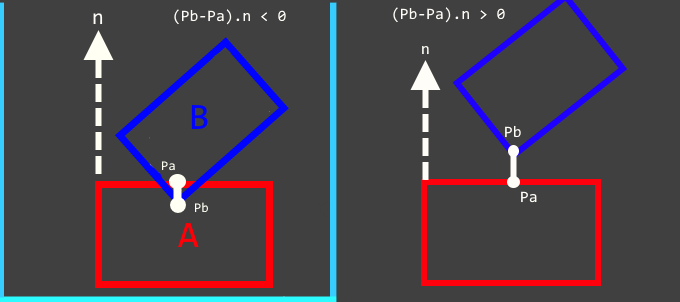
Let’s call the contact point of B Pb and the contact point of A Pa.
When we try to separate this collision along with the collision normal, what happens to Pb and Pa when the collision is separated? You can see visually that the moment that the collision is resolved when the vector created by Pb and Pa is pointing along with the collision normal.
In other words, we have a CONSTRAINT c where the dot product between (Pb-Pa) and the collision normal ’n’ must be bigger and or equal to zero.
C: (Pb-Pa) . n ≥ 0
Now at this point, you might be inclined to think that we can simply resolve the collision by simply changing the positions of the colliders in the direction of the collision normal, but there a few problems with this:
Problems with solving at the position level
To my knowledge, at the moment of writing, most collision solvers for rigid bodies are mostly velocity based. This means that we try to find the velocity necessary to resolve the collision at the next physics time step. Here are a few problems that one might face when solving at the position level:
- Potentially creating new collisions
Moving a rigidbody in order to resolve a collision may cause it to create new collisions and may even “invalidate” the already detected collisions. This means we would have to run the collision detection phase again (which may not be something we want). This brings us to the next problem:
2. Problems with stacking
When we have rigid bodies that are in contact with more than one rigidbody at once (Like a pile or stack of bodies), it will continuously go from penetrating one rigidbody in one time step, to penetrating another rigidbody in another time step. This will cause visible jitter on the rigidbody.
3. The velocity problem
Keep in mind that moving the rigidbodies still does not change its velocity. This means that in the next time step, the same collision will happen again.
SOLVING THE CONSTRAINT AT THE VELOCITY LEVEL
So with that out of the way let’s try to solve this constraint at the velocity level. As hinted previously, the idea behind a velocity level collision solver is that we are looking for the linear and angular velocities that will resolve the collision we found.

We can put these values on a 12x1 matrix that we will call delta-v.
The first 3 values represent the linear velocity we need to add to rigidbodyA, we will call this va.
The next three values represent the angular velocity that we need to add to rigidbodyA, we will call this wa.
And of course, the same concept works for rigidbodyB. There is a certain linear and angular velocity that we need to add to stop the bodies from colliding denoted as vb and wb.
So how do we find delta-V? Well, we can start by finding the velocity constraint of our collision.
Let’s work with what we have. We already know the position constraint, we now need to find some sort of relation between position and velocity. Luckily, there is one. We know that the rate of change of the position of our colliders is its velocity.
Or, in other words, what we can do is we can find the derivative of the position constraint over time
The problem now is that we are now dealing with deriving the product of elements that both change over time. If you remember Figure 5, we know that both Pa and Pb change over time as the bodies move away from each other.
In order to find the time derivative, we need to use the product rule of differentiation
which states that:
The derivative of the product of f and g with respect to x is equal to the derivative of f multiplied by g plus f multiplied by the derivative of g

Therefore the time derivative of our position constraint is:
C: (Pb-Pa) . n ≥ 0
Cdot : [ d/dt (Pb — Pa) ]. n + (Pb — Pa) . d/dt [n]
Now let's expand this,
We need to find the rate of change Pa, Pb, n over time
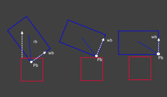
Let's remember what Pb initially stands for,Pb is a point on a rigidbody. It moves with the rigidbody and rotates around its centroid, so the rate of change of Pb over time would be:
d/dt Pb = Vb + Wb x Rb
the velocity of Va plus the cross product of wb and rb. Or in other words, its linear velocity and its angular velocity
The same can be said for Pa.
d/dt Pa = Va + Wa x Ra
And as for n, we must also remember that this collision normal is attached to a face or an edge of the reference collider. In Figure 5, our current collision normal is attached to the edge of ‘ab’. This means that it changes over time depending on the angular velocity.
n = Na x Wa
So we can then put it all together
Cdot : [(Vb + Wb x Rb — (Va + Wa x Ra) ) ]. n + (Pb — Pa) . [Na x Wa]
Now you can see that things are getting quite hairy but there is a simplification we can make.
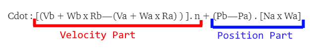
We need to remember that our goal is to shift the velocities of our objects. And looking at our constraint, We can see that the first part is the velocity constraint and the second part is the position constraint.
What we could do is we could simply ignore this part.
Cdot : [(Vb + Wb x Rb -(Va + Wa x Ra) ) ]. n
So now that we have the velocity constraint defined, you might notice something quite interesting.
Our velocity constraint coincidentally contains all the elements of delta-V. We have va, wa, vb, wb.
Remember, that we are looking for a 12x1 matrix with va, vb, wa, wb. Perhaps if we could somehow re-arrange the velocities like this:

We could actually insert delta-v into our velocity constraint.
Cdot : Vb.n + (Wb x rb).n — (Va).n — (Wa x ra).n
When we try to do this, Vb.n and Va.n can be easily separated, but what about (Wb x rb).n and (Wa x ra).n?
This is where the triple product identity comes in:
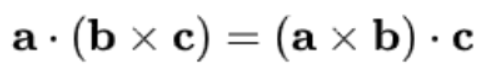
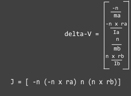
Using this identity we can now isolate delta-V.
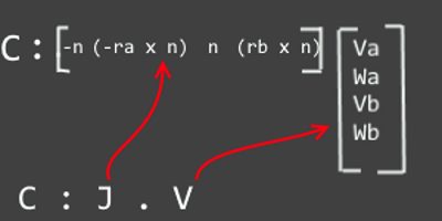
From now on, let's call the first matrix J and the velocity part V.
Now delta-v fits quite neatly into our constraint. It also adds up quite nicely in terms of intuition. We have a certain function where J is multiplied by V. And we need to add a certain delta-V to resolve it.
C : J(V + delta-V)
Unfortunately, We still don't know what the values of delta-V are so let's get that.
Remember, Every component of delta-V is a vector. And as we know, a vector has a certain magnitude and direction. So that’s what we need to do next we need to find the magnitude and direction of every component of delta-V.
Before we get to that, there’s actually a problem we need to solve.
How do we make sure that this “shift” in velocity is physically based? For example, assume a situation where a light tennis ball hits a heavier bowling ball, one would expect that the tennis ball would bounce off and barely move the bowling ball. The reason for this is because the mass of the object does matter. So what we need to do is find something that takes into account both mass and velocity. And this “thing”, as you might have guessed from the title of the article, is an impulse.
We know that linear momentum is equal to
P = m.v
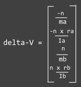
mass of the object, multiplied by its velocity. So we can now add that to delta-v. Keep in mind that Pa is negated.

We can then do the same for angular velocities. Since we know that angular velocity (W) is equal to the angular momentum (L) divided by the moment of inertia (I).
L = I W
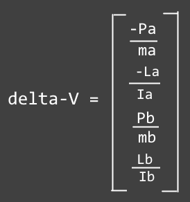
Now keep in mind the problem of finding the magnitude and direction of va,vb,wa,wb hasn't changed. We are now looking for the magnitude and direction of Pa,Pb,La,and Lb.
So how do we do that? We don’t necessarily know the length of these vectors but we actually already know the directions. Remember, we might be solving the problem on the velocity level, but the direction in which we resolve the collisions actually has not actually changed.
For example, the direction of impulseB and would still be the collision normal. The inverse is true of impulseA.
and in the case of the angular momentum of B and A, it would be the vector perpendicular to ra/rb and the collision normal, the same concept applies for the angular momentum of B.
With this info, we can now replace Pa, Pb, La, and Lb with the appropriate directions.
We still don’t know the scalar parts of these vectors. But you might have noticed something interesting. somehow the 12x1 matrix J, which we have mostly ignored so far has suddenly reappeared in our formula.
Let's first make this a bit tidier by putting the masses into its own matrix. For the sake of making it tidier. Let's call this matrix the inverse mass matrix. Keep in mind we haven't changed anything, we’ve just moved the mass part of our equation into its own matrix.
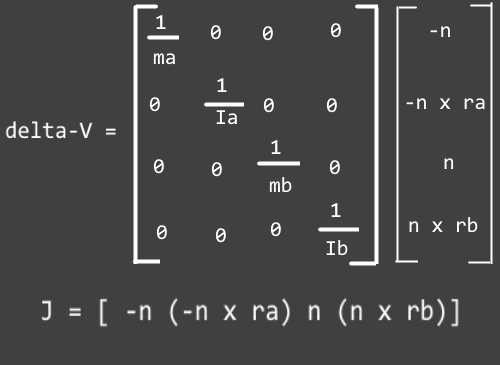
But going back to the reappearance of the matrix J, This actually implies something very interesting. We initially thought that a,b,c,d are different values. But they are actually the same value. Let’s call this value lambda.
And this might confuse you, what does the re-appearance of the matrix J have to do with the values of a,b,c, and d being the same value?
Here’s an interesting analogy that I will borrow from Allen Chou’s explanation of sequential impulse:
Let's go back to the idea of expressing collision as a constraint.
C: J.V
as I have mentioned before, we have a velocity constraint that outputs a singular number. If the number is positive our bodies are separating from each other, if it's negative they are colliding with each other.
This behavior is oddly similar to finding the distance of a point to a plane.
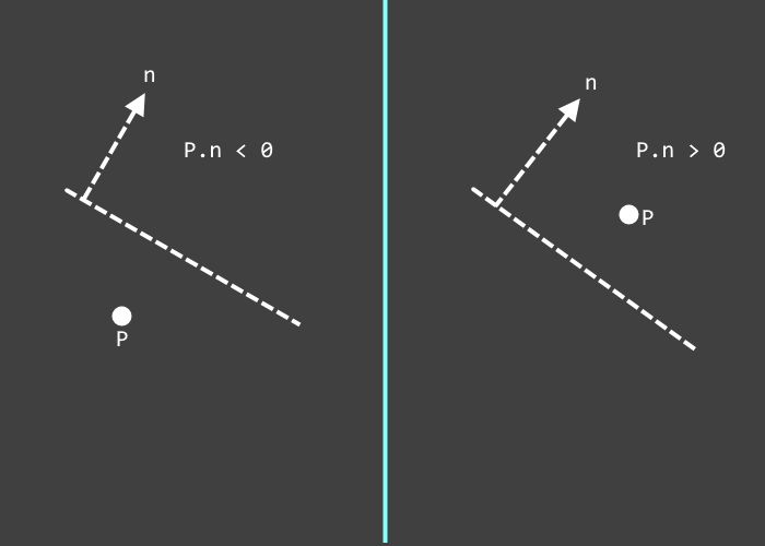
And we actually know how to get the closest distance of a point to a plane. We can do this by adding the point by the normal of a plane multiplied by a single scalar value that represents the closest distance of the point to the plane.
delta-V = normal * dist
normal.(point + delta-V) = 0
The idea is that we can do the exact same thing with our constraint
delta-V = J^T * lambda
C: J.(V + delta-V) =0
But as mentioned before, in order to keep the velocities physically-based we still need to multiply the mass matrix
delta-V = M^-1 * J^T * lambda
Quick tangent before we continue: Although this isn’t necessarily important in order to understand sequential impulses, it's a good thing to mention that we now see that the J matrix isn’t just the ‘leftover’ variables we get from isolating the linear and angular velocities. In our simulation, the collision normal of 2 colliding objects changes over time, and if we were to graph it out we might get a relatively non-linear line.
but the J matrix basically gives a “snapshot” of a small part graph and tells us the direction we need to use to separate the colliding bodies. In a broader sense, the idea of a matrix that gives a “snapshot” of a certain point in a complex transformation isn’t new; in fact, there is a formal name to it. It's called the jacobian matrix.
But with that out of the way let's solve our next problem: Finding the value of lambda.
FINDING LAMBDA (AND KNOWING WHY WE NEED TO CLAMP IT)
Let's go back to our constraint. We have a constraint C: J.V that needs to be bigger or equal to zero
C: J.V ≥ 0
And we have a delta-V we would like to that to shift our velocities
J(V + deltaV) = 0
but now we know that value of delta-V and we can put that into our equation
deltaV = M^-1 * J^T * lambda
J(V + M^-1 * lambda * J^T) = 0
JV + J M^-1 lambda * J^T = 0
lambda = (JV )/ ( J M^-1 * J^T )
With this lambda, we finally know everything we need to calculate deltaV.
One question that might come to mind is: does it matter if lambda is positive or negative, and I think it's not surprising that the answer to this is yes, it does actually matter because if lambda is negative it would actually shift the velocities away that brings them closer together instead of further.
And one might be tempted to first clamp the lambda but this is not something we actually want.
Let's go look at a situation where we have 2 contact points instead of one.
One thing to remember is that we are not solving our contacts at the same time (I’ll explain more about this later). Let’s say in this situation the impulses added by p1 are too strong causing it to bounce. This might be okay in some situations but if for example a user intentionally sets the restitution of this RB to 0. We wouldn’t want this to happen. It then makes sense that the next impulse needs to actually pull the rigid body closer to whatever it currently colliding with.
But one thing we need to do is to clamp the accumulated impulses. Because although we know that a singular negative lambda is fine, the TOTAL lambda should not be negative because that would mean that in the next frame the bodies would get closer instead of further.
But since I’ve just mentioned the idea of having more than one contact. This might make you wonder, in the case where there are multiple rigidbodies, and multiple contact points, like a stack of boxes lets say,how do we solve such a collision?
The answer to that is really simple.
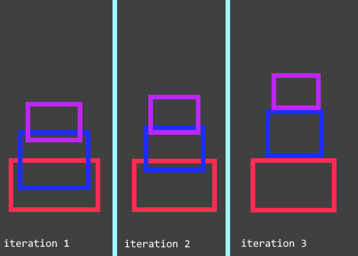
We simply go through all contacts and resolve the collisions for a number of iterations. The idea is that the more iterations we do, the closer we are to the “correct” velocities.
But you might be interested in why this actually works and why does iterating through our contact points actually causes our simulation to converge. Why do you need multiple iterations in order for the solution to converge? Why can’t you just do it once?
Well before we get to that there’s actually one concept we need to understand and that is the idea of sequential impulse as an MLCP.
SEQUENTIAL IMPULSE AS AN MLCP
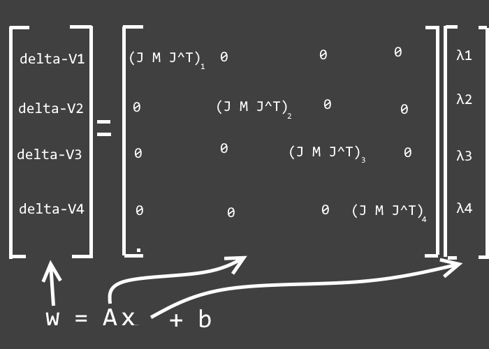
In the case where a 3D Box is lying on a plane, we would have 4 contact points instead of one. Because of this, we would have 4 delta-Vs
delta-V1 = (J M J^T)1 * lambda1
delta-V2 = (J M J^T)2 * lambda2
delta-V3 = (J M J^T)3 * lambda3
delta-V4 = (J M J^T)4 * lambda4
When we had only one contact point, we only needed to make sure that lambda1 is above zero. And we were able to do that by simply going through the calculation. But now there are four of them. And that’s a problem because what if resolving one contact will actually cause a collision another one?
This problem can actually be more formally expressed. We would like all the values of lambda to be positive, we also actually want delta-V to be positive because that would mean that the constraint is being resolved. Our problem at the very core of it is an MLCP, a mixed linear complementarity problem.
Let's break that down,
A Linear Complementarity Problem is a very specific problem when we have a 1xn matrix, which we will call w, an n x n matrix A and a 1xn matrix x, where we would like each element of w to be positive and all elements of x to be positive
[w] = Ax + b
And the mixed in the mixed linear complementary problems basically adds certain bounds to the problem
for example, x can be bounded by a min value and a max value.
Now you might have noticed that our problem can be expressed as an MLCP.
So now we know that our problem at the very core of it, is an MLCP, the next step is to actually solve the MLCP. And there are actually quite a few methods of doing so but we are going to be focusing on a very specific one called the Projected Gauss-Seidel.
Let's break that down,
At the very core of it, the Gauss-Seidel method involves taking a set of linear equations and solving them by making a guess at the values we are looking for and then using them to find a better guess. We do this until we converge on a single answer.
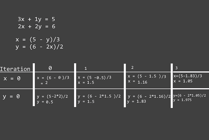
Here’s an example, let’s say we have the following linear equations. We would like to know the values of x and y. What we can do is get the equations of x and y . We then make an initial guess for x and y. Then, every time we get a new value, we use it on the next iteration. And we can see that if we were to do this a number of times we slowly converge to an answer.( x = 1 , y = 2)
And that's exactly what we are doing with Projected Gauss-Seidel does.
We have a set of linear equations
delta-V1 = (J M J^T)1 * lambda1
delta-V2 = (J M J^T)2 * lambda2
delta-V3 = (J M J^T)3 * lambda3
delta-V4 = (J M J^T)4 * lambda4
We find the equation for each value we are looking for, in our case, we are looking for the value of lambda:
lambda = -(J.V)/(J M J^T)
We use an initial guess, which in our case would be the velocity of the rigid bodies before the collision.
We then solve them iteratively. We also then need to clamp the total lambda, hence the “projected” in PGS.
Now if you look back at sequential impulse at then to projected gauss seidel, you might notice that they are basically the same thing. In both cases, we are looking for a lambda, or an ‘X’, we are clamping it and then applying it to our bodies. And the only difference is that in Sequential Impulses, we are applying these changes explicitly to our rigid bodies and the MLCP is implicit. On the other hand, in the case of Projected Gauss-Seidel, we are creating an explicit A matrix, an x matrix, and a w matrix.
And that’s about it for my attempt at explaining sequential impulses and why it works. If you’re looking for an even deeper explanation of Sequential Impulse and or PGS, I’ve linked a few sources that have helped me make this article. But until then, I’ll see you at the next one!
Sources and acknowledgments:
[1] Erin Catto’s paper “Iterative Dynamics with Temporal Coherence” and GDC talks were definitely essential in helping me understand PGS and sequential impulse.
[2] Helmut Garstenauer’s master thesis “A Unified Framework for Rigid Body Dynamics” gave a good primer for MLCPs and introduced me to constraint-based collision resolution.
[3]Allen Chou’s explanation of Sequential Impulse was what introduced me to sequential impulse and inspired me to make my own explanation.
